

Sales reports, payroll, stock lists and budgets in Malaysia often live in Excel. The people who know their formulas finish in minutes what takes others an afternoon.
Quick answer: Excel formulas start with an equals sign. SUM, AVERAGE, IF, SUMIF, COUNTIF and XLOOKUP (or VLOOKUP in Excel 2016 or 2019) cover everyday reports. For a rate, divide and format as a percentage. For change, use (new−old)/old when the old value is not zero. TODAY() updates when Excel recalculates. Always test AI-written formulas on known rows first.
This cheat sheet covers the Excel formulas you will actually use at work, with a plain explanation and an example for each. At the end of every section there is a prompt you can paste into ChatGPT, Gemini, Claude or Microsoft Copilot to get the formula written for your own data. Use a short, anonymised sample — not a real payroll or customer list.
Last fact-checked: 10 November 2026 (against Microsoft’s public Excel documentation — not a first-hand Excel test).
Quick Reference Excel Formulas List
Start an Excel formula with an equals sign. A formula is the whole expression; a function is a named operation such as SUM, while operators are symbols such as - or *. Where a worked result is shown, the sample inputs are given in that row.
| What you want to do | Copyable formula | Expected result |
|---|---|---|
| Add numbers | =SUM(B2:B10) | The total of the numbers from B2 to B10 |
| Subtract | =B2-C2 | If B2 is 100 and C2 is 80, the result is 20 |
| Multiply | =B2*C2 | If B2 is 10 and C2 is 25, the result is 250 |
| Divide | =B2/C2 | If B2 is 100 and C2 is 20, the result is 5 |
| Work out a percentage | =B2/C2 | If B2 is 25 and C2 is 100, this shows as 25% after percentage format |
| Percentage change | =(C2-B2)/B2 | If B2 (old) is 100 and C2 (new) is 120, this shows as 20% after percentage format |
| Average | =AVERAGE(B2:B10) | The average of the numbers in that range |
| Count numbers | =COUNT(B2:B10) | How many cells contain numbers or dates |
| Count matching items | =COUNTIF(A2:A100,"Penang") | How many rows in A2:A100 say Penang |
| Add matching items | =SUMIF(A2:A100,"Penang",C2:C100) | The total of column C where column A is Penang |
| Check a condition | =IF(B2>=50,"Pass","Fail") | “Pass” if B2 is 50 or more; otherwise “Fail” |
| Look up a value | =XLOOKUP(E2,A2:A100,C2:C100,"Not found") | The matching value from column C, or “Not found” |
| Today’s date | =TODAY() | The current date, updated when Excel recalculates |
| Years between two dates | =DATEDIF(B2,C2,"Y") | The complete years from the date in B2 to the date in C2 |
| Join text | =A2&" "&B2 | First name and last name with a space |
| Remove extra spaces | =TRIM(A2) | The text with extra spaces removed |
| Hide errors | =IFERROR(B2/C2,"Check") | The result of B2/C2, or “Check” if that would be an error |
| Growth rate per year | =(C2/B2)^(1/D2)-1 | If B2 is 1,000,000, C2 is 1,500,000 and D2 is 3, the result is about 14.5% |
Basic Maths Formulas
SUM formula in Excel
The SUM formula adds up a range of numbers.
=SUM(B2:B10) adds every number from cell B2 to B10.
You can also add separate cells or ranges in one go, like =SUM(B2:B10, D2:D10). The fastest way to use it on Windows is to select the cell below a column of numbers and press Alt and = together. Excel writes the SUM formula for you. On a Mac, the official AutoSum shortcut is Shift + Command + T.
Excel minus formula (subtraction)
Excel does not have a MINUS function. You subtract with the minus sign.
=B2-C2 takes the value in C2 away from B2. If B2 is 100 and C2 is 80, the result is 20.
To subtract several cells from one number, you can write =B2-SUM(C2:E2). This is cleaner than =B2-C2-D2-E2 and less likely to go wrong when you add columns later.
Excel multiply formula
Use the asterisk to multiply.
=B2*C2 multiplies the values in B2 and C2. This is how most people work out a line total, such as quantity times unit price. If B2 is 10 and C2 is 25, the result is 250.
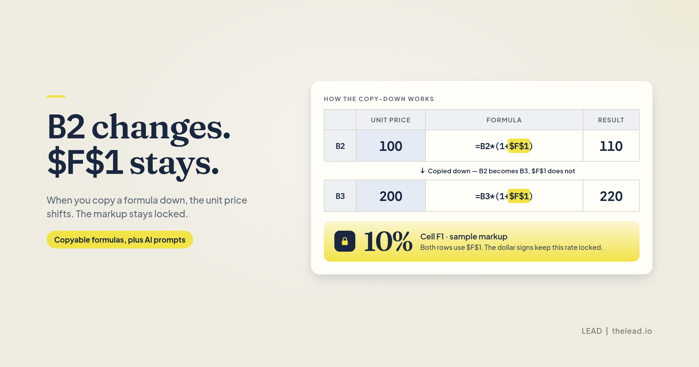
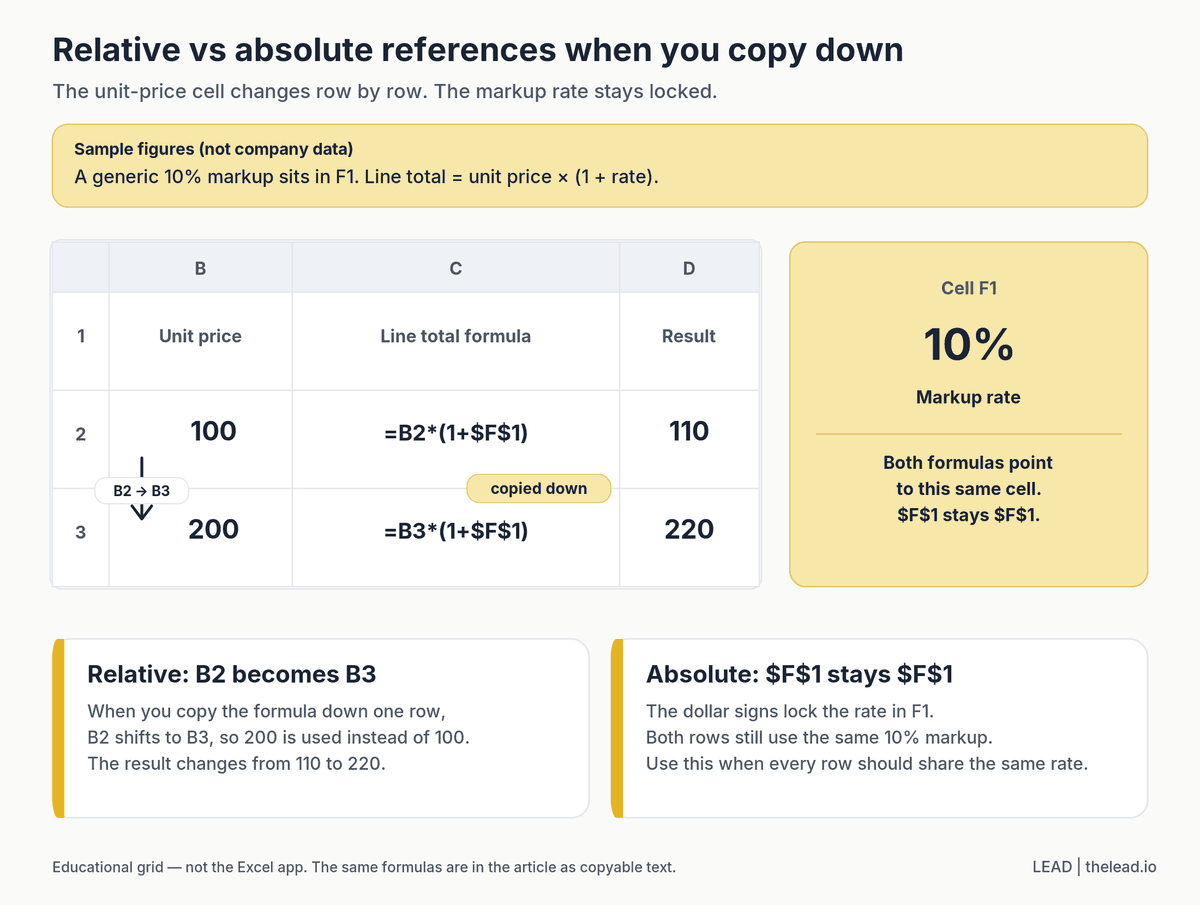
To multiply a whole column by a fixed rate, such as a 10% markup on every unit price, lock the cell that holds the rate with dollar signs. If the rate in F1 is 10% and B2 is 100, write =B2*(1+$F$1). The result is 110. Copy it down to the next row, where B3 is 200, and it becomes =B3*(1+$F$1), which is 220. The dollar signs stop Excel from shifting F1 as you copy. This is a generic markup example, not tax advice — use the rate that actually applies to your prices.
Divide in Excel
Use the forward slash. =B2/C2 divides B2 by C2. If B2 is 100 and C2 is 20, the result is 5.
If C2 might be empty or zero, do not quietly hide that with =IFERROR(B2/C2,0), because a zero can look like a real answer and hide a data problem. A clearer option is =IFERROR(B2/C2,"Check"), or an IF that tests whether C2 is greater than zero before you divide.
Average formula in Excel
=AVERAGE(B2:B10) returns the average of the numbers in that range. Empty cells are ignored, but cells with zero are counted, so check your data if the average looks low.
If you need the middle value instead, which is better when a few very large numbers skew the result, use =MEDIAN(B2:B10).
AI prompt to try. “I have quantities in column B and unit prices in column C, from row 2 to row 200. Write an Excel formula for column D that multiplies them, and another formula at the bottom that totals column D. If a row is blank, leave column D blank.”
Percentage Formulas in Excel
Basic percentage
To find what percentage one number is of another, divide and then format the cell as a percentage.
=B2/C2 gives a decimal like 0.25. On a US keyboard layout, press Ctrl + Shift + % to show it as 25%. That is Control, not Command, on a Mac as well. Shortcuts on other keyboard layouts may differ.
Percentage of a total
If B2 is one salesperson’s sales and B12 is the team total, use =B2/$B$12. The dollar signs lock the total so you can copy the formula down the column.
Percentage change
To compare this month with last month, use =(C2-B2)/B2, where B2 is the old value and C2 is the new one. Format it as a percentage. A negative result means a drop. This only works when the old value is a meaningful number other than zero. A zero or blank starting value will give an error or a misleading result, and a negative starting value can also be hard to interpret.
Increase or decrease a number by a percentage
To add 10% to a price in B2, use =B2*(1+10%). To take 15% off, use =B2*(1-15%).
AI prompt to try. “Column B has last month’s sales and column C has this month’s sales for 50 branches. Write a formula for column D that shows the percentage change, and tell me how to highlight any branch that dropped more than 10%. If last month’s sales are zero or blank, show a message instead of an error.”
Logic Formulas
IF formula in Excel
IF checks whether something is true and returns one result if it is and another if it is not.
=IF(B2>=50,"Pass","Fail")
You can combine conditions. =IF(AND(B2>=50,C2="Yes"),"Eligible","Not eligible") only returns Eligible when both conditions are met. Use OR instead of AND when either condition is enough.
For more than two outcomes, IFS is easier to read than several IFs inside each other.
=IFS(B2>=80,"A",B2>=65,"B",B2>=50,"C",TRUE,"F")
IFS is available in Excel 2019, Excel 2021, Excel 2024 and Microsoft 365. It is not in Excel 2016, so use nested IF formulas if the file must open in that version.
IFERROR
IFERROR replaces an error with something more useful, like a blank or a short message. For a lookup, =IFERROR(XLOOKUP(E2,A2:A100,C2:C100),"Not found") shows “Not found” instead of #N/A. A cleaner option in Microsoft 365 or Excel 2021 or later is to use XLOOKUP’s own if_not_found argument, like =XLOOKUP(E2,A2:A100,C2:C100,"Not found").
Avoid returning 0 for every error, especially in divisions, because that can hide missing or zero values.
AI prompt to try. “Write an Excel IF formula that gives a 5% bonus if sales in B2 are above RM50,000, 3% if they are above RM30,000, and nothing otherwise. Return the bonus amount in ringgit.”
Counting and Conditional Totals
COUNT and COUNTA
=COUNT(B2:B100) counts cells with numbers, including dates (Excel stores dates as numbers). It does not count plain text.
=COUNTA(A2:A100) counts cells that are not empty, including text. It also counts error values and formulas that look blank because they return an empty string (""). That means a formula-generated blank is still counted. Use COUNTA to count names, orders or other text entries, but check for those hidden blanks if the count looks high.
COUNTIF
COUNTIF counts the cells that match a condition.
=COUNTIF(A2:A100,"Penang") counts how many rows say Penang. =COUNTIF(C2:C100,">1000") counts values above 1,000.
SUMIF formula in Excel
SUMIF adds up numbers that match a condition. It takes three parts, which are the range to check, the condition, and the range to add.
=SUMIF(A2:A100,"Penang",C2:C100) adds the sales in column C for every row where column A says Penang.
SUMIFS for more than one condition
SUMIFS works the same way but lets you add several conditions. Note that the range to add comes first.
=SUMIFS(C2:C100,A2:A100,"Penang",B2:B100,"Laptop") adds sales of laptops in Penang only.
AI prompt to try. “My sheet has region in column A, product in column B and sales in column C. Write a SUMIFS formula that totals sales for each region and product combination, and suggest how to lay out the summary table.”
Lookup Formulas
XLOOKUP
XLOOKUP finds a value in one column and returns the matching value from another. It is available in Microsoft 365 and Excel 2021 or later. Excel 2016 and Excel 2019 do not have it, so use VLOOKUP in files that must work in those versions.
By default, XLOOKUP looks for an exact match. The fourth argument is what to show if nothing is found, not a VLOOKUP-style approximate-match flag.
=XLOOKUP(E2,A2:A100,C2:C100,"Not found")
This looks for the value in E2 within column A and returns the matching value from column C. If nothing matches, it shows “Not found”.
VLOOKUP
If you work with an older version of Excel, use VLOOKUP.
=VLOOKUP(E2,A2:C100,3,FALSE)
The 3 tells Excel to return the third column of the range, and FALSE means exact match. Always use FALSE unless you know you need an approximate match.
AI prompt to try. “I have an employee list with staff ID in column A and department in column D on a sheet called Staff. On another sheet I have staff IDs in column A. Write an XLOOKUP that brings in the department and shows ‘Missing’ if the ID is not found. I use Excel for Microsoft 365.”
Date Formulas
Excel formula for today’s date
=TODAY() shows today’s date. =NOW() shows the date and time. Both update when Excel recalculates — including when you open the file if calculation is set to Automatic, and also after other changes that trigger a recalc. If the workbook is set to Manual calculation, they may not update when you expect.
If you need a date that does not change, press Ctrl + ; on Windows to type today’s date as a fixed value. On a Mac, that official shortcut is also Control + ;.
Days between two dates
Subtract one date from the other. =C2-B2 gives the number of days. For working days only, use =NETWORKDAYS(B2,C2). NETWORKDAYS counts the start and end dates if they fall on a workday, and it treats Saturday and Sunday as the weekend by default.
Malaysian public holidays are not applied automatically. Add your own holiday list as a third part, like =NETWORKDAYS(B2,C2,H2:H20). If your weekend is not Saturday–Sunday, use NETWORKDAYS.INTL instead and set the weekend pattern.
Years of service or age
=DATEDIF(B2,TODAY(),"Y") returns the complete years between the date in B2 and today. Use "M" for complete months or "D" for days. DATEDIF does not appear in Excel’s formula suggestions, but it works. Microsoft warns that it can calculate incorrect results in some cases, and you should not use the "MD" unit.
Add months to a date
=EDATE(B2,3) returns the date three months after B2. This is handy for contract renewals and probation end dates.
AI prompt to try. “Column B has staff join dates. Write formulas to show years of service, the probation end date six months after joining, and a flag that says ‘Review due’ if the probation end date is within the next 14 days. I use Excel for Microsoft 365.”
Text Formulas
Join text
=A2&" "&B2 joins a first name and last name with a space. To join a whole range with a separator, use =TEXTJOIN(", ",TRUE,A2:A10). TEXTJOIN is available in Excel 2019, Excel 2021, Excel 2024 and Microsoft 365. It is not in Excel 2016.
Clean up text
=TRIM(A2) removes extra spaces. =PROPER(A2) capitalises each word. =UPPER(A2) and =LOWER(A2) change the case of the whole text.
Pull part of a text
=LEFT(A2,3) returns the first three characters. =RIGHT(A2,4) returns the last four. In Microsoft 365 and Excel 2024, =TEXTBEFORE(A2,"@") returns everything before the @ in an email address. TEXTBEFORE is not listed for Excel 2016, 2019 or 2021.
CAGR Formula in Excel
CAGR stands for compound annual growth rate. It tells you the average yearly growth between two values, which is useful for revenue, investments and headcount.
=(C2/B2)^(1/D2)-1
Here B2 is the starting value, C2 is the ending value and D2 is the number of years. Format the result as a percentage. If revenue grew from RM1 million to RM1.5 million over 3 years, the CAGR is about 14.5%. This assumes a positive starting value, a meaningful ending value and a number of periods greater than zero. A zero or negative starting value will give an error or a result that is not a meaningful CAGR.
You can also use the RRI function, which gives the same kind of answer: =RRI(D2,B2,C2).
Keyboard Shortcuts That Save Time
These official shortcuts use a US keyboard layout. Keys on other layouts may differ. On a Mac, do not swap Command for Control on every shortcut — several of these still use Control.
| What it does | Windows | Mac |
|---|---|---|
| Insert SUM (AutoSum) | Alt + = | Shift + Command + T |
| Format as percentage | Ctrl + Shift + % | Control + Shift + % |
| Insert today’s date as a fixed value | Ctrl + ; | Control + ; |
| Cycle dollar signs on a selected reference while you edit a formula | F4 | Command + T, or F4 |
| Show all formulas instead of results | Ctrl + ` | Control + ` |
| Fill down from the cell above (or the top of the selection) | Ctrl + D | Control + D, or Command + D |
F4 (or Command + T on a Mac) only cycles the dollar signs when you have selected a cell reference inside the formula bar. Outside that, F4 repeats the last action.
Keyboard shortcuts in Excel (Microsoft)
How to Get AI to Write Excel Formulas for You
You do not need to memorise every formula. AI tools are very good at writing Excel formulas, as long as you describe your sheet clearly and you do not paste real company data into a consumer tool. A good prompt has four parts.
- Your Excel version, since older versions do not have XLOOKUP, IFS or some text functions
- What is in each column, including the column letters and the first and last rows
- What you want the result to be, in plain words
- Any rules or exceptions, such as ignoring blanks or showing a message if nothing matches — then test the formula on a few rows where you already know the answer
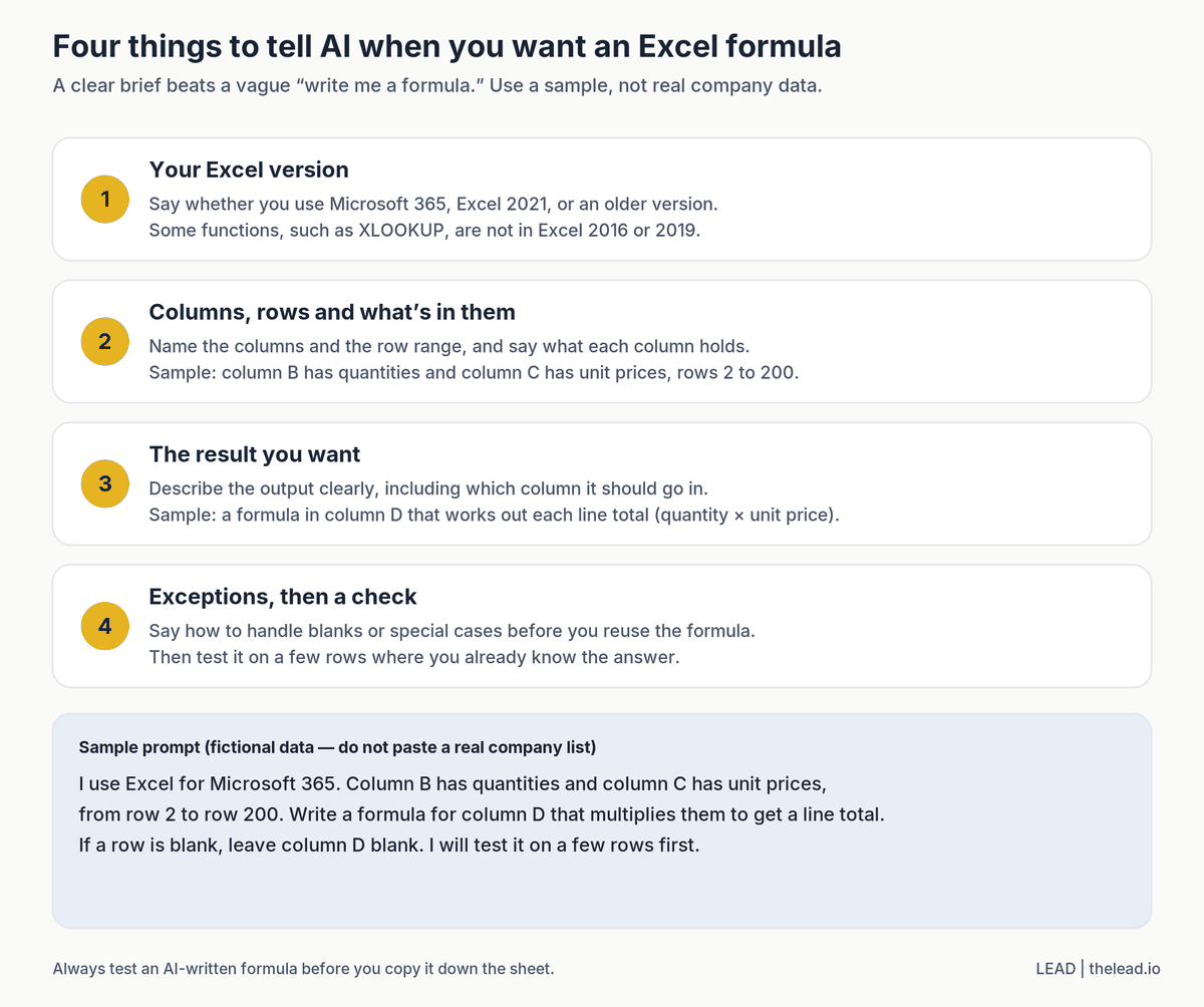
Here is a full example you can adapt. It uses fictional sample data, not a real invoice list.
“I use Excel for Microsoft 365. Column A has invoice dates, column B has customer names and column C has invoice amounts, from row 2 to row 500. On a new sheet I want a table with one row per customer and one column per month for 2026, showing the total invoiced. Write the formula for the first cell and explain how to fill the rest.”
If you use Microsoft 365 with an eligible Copilot licence, you can ask Copilot inside Excel through the Copilot pane. Microsoft ended the =COPILOT() in-cell function on 14 September 2026; it was a preview feature, and cells that still contain it now return a #NAME? error. Use the pane for generative tasks such as summarising or classifying text. For totals, lookups and other calculations that should come out the same every time, keep using ordinary Excel formulas, and always test an AI-written formula on a few rows where you already know the answer before you copy it down the sheet.
Go Further Than Formulas
Formulas save minutes. Automation saves hours. Once you know how to describe a task clearly to AI, the next step is to work more confidently with larger datasets, dashboards and, later, automated reports.
Our AI for Data Science Certification is a two-day flagship for people who already work in Excel and want to go further with data and dashboards. It’s HRDC-claimable for eligible employers. If you later want to automate reporting workflows across tools, see our n8n training in Malaysia. Aside from that, we frequently run one-day masterclasses, workshops, and other AI courses that you can find in our certifications hub.
Frequently Asked Questions
What are the most important Excel formulas to learn first?
Start with SUM, AVERAGE, IF, SUMIF, COUNTIF and XLOOKUP (or VLOOKUP if you are on Excel 2016 or 2019). These cover a large share of everyday reports, from totals and averages to conditions, filtered totals and lookups.
Is there a minus formula in Excel?
There is no MINUS function. Use the minus sign, like =B2-C2. To subtract a range, use =B2-SUM(C2:E2).
How do I calculate a percentage in Excel?
Divide the part by the total, like =B2/C2, then format the cell as a percentage with Ctrl + Shift + % (Control + Shift + % on a Mac, on a US keyboard layout).
What is the Excel formula for today’s date?
=TODAY(). It updates when Excel recalculates, not only when you open the file. If calculation is set to Manual, it may not update until you recalculate. Press Ctrl + ; (Control + ; on a Mac) if you want a fixed date instead.
Why does my formula show as text instead of a result?
Either the formula does not start with an equals sign, or the cell is formatted as Text. Change the format to General and re-enter the formula.
Should I use VLOOKUP or XLOOKUP?
Use XLOOKUP if you have Microsoft 365 or Excel 2021 or later. It is simpler, can look left as well as right, and handles missing values more neatly. Use VLOOKUP only when the file must work in older Excel versions, such as Excel 2016 or 2019.
Can ChatGPT write Excel formulas?
Yes. ChatGPT, Gemini, Claude and Copilot can all write Excel formulas. Describe your Excel version, columns, rows and the result you want, use a short anonymised sample rather than real company data, and always test the formula on a few rows first.
What is the difference between COUNT and COUNTA?
COUNT tallies cells with numbers, including dates. COUNTA tallies non-empty cells, including text, errors, and formulas that return an empty string (""), so a formula that looks blank can still be counted.
Why isn’t NETWORKDAYS skipping my holidays or Friday–Saturday weekend?
NETWORKDAYS treats Saturday and Sunday as the weekend by default, and it counts the start and end dates if they are workdays. Malaysian public holidays are not built in — add them as the third argument. If your weekend is not Saturday–Sunday, use NETWORKDAYS.INTL.
I am on a Mac. Can I just use Command instead of Ctrl?
No. Several official Excel for Mac shortcuts still use Control, including percentage format (Control + Shift + %), a fixed today’s date (Control + 😉 and show formulas (Control + `). AutoSum on a Mac is Shift + Command + T. See the shortcut table above.
Does Excel still have a COPILOT function I can type into a cell?
No. Microsoft ended the =COPILOT() function on 14 September 2026. It was a preview feature. Existing formulas now return #NAME?. If you have an eligible licence, use the Copilot pane in Excel instead, and keep ordinary formulas for calculations that should be exact.
0 Comments